Linear regression is an approach for predicting the relationship between
a single dependent variable y and one or more explanatory variables (or
independent variables) usually called X#. (To predict which of
several categories y falls in, instead of finding a linear prediction of
y, see Logistic Regression). This linear
prediction is just like all those algebra problems in the form Y = mX + b
that you did in high school. You can see an example of it on this page:
https://stackblitz.com/edit/minml?file=index.js
The problem with that is it only allows one input (the X) (and it only fits a straight line). Actual Linear Regression supports many inputs. It's still basically Y = mX + b except with more than one X like Y = b +
m1X1 + m2X2 ... and to simplify
the math and allow the use of matrix multiplication, we assume an
X0 which is alway set to 1, and change b into m0 and
all the m's into theta or o. The result is:
y = o0x0 +
o1x1 +
o2x2 ...
which can be expressed via matrix math as
OTX where O is a vector of all
the o's e.g. [o0,
o1, o2, ... ] which
used to be all the m's, except o0 which used
to be the b, and X (note it's uppercase) is a matrix of all the values of
x e.g. [x0 , x1 , x2 , ...] where
x0 is always 1. Note T means Transpose or turn the vector into
a 1x# matrix so it can be multiplied by X. So
OTX just takes each element of O
and multiplies it times each element of X and adds up the result which is
y.
O becomes the parameters which shape different values of
X into a prediction y. (Note O and X are uppercase, y is
lowercase by convention that O and X are matrices i.e. arrays
and y is a scalar i.e. a single number)
The trick is to find a set of values for O such that for
every given X, y is a valid prediction. Or rather, given a training set of
values for X, we find values for O such that the resulting
values of y are as close as possible to those given in the training set.
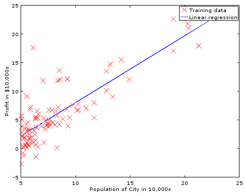
Then we can apply new values of X, and hope that y will be predictive. Here
is an example of a linear fit to a set of sample data:
In order to find better values for O, we need to understand
how wrong our value of y is for ALL the values of X in the training set.
A key point is that there may be values of O which work
for ONE value of X but not for others. So when we evaluate our current
O, we must sum the error for all the given values (or sets
of values) of our current guess. To do this, we create a cost function which
compares the difference between the desired outcome y and the actual outcome
OTX and average that over the number of samples
in the training set, m. (m is used by convention to represent the number
of samples).
The Mean Squared Error
(MSE)^ function
is commonly used. This is the error squared
(OTX - y)2 then the mean of that;
the sum of the error squared, divided by the number of samples. We will actually
compute half the MSE for reasons which will become clear later (hint:
derivative).
s = 0;
for (j = 0; j<m; j++) { // m = number of samples, length of y and 2nd dim of X
  for (i = 0; i<p; i++) { // p =number of parameters, length of theta
    hyp = theta[i] * X[j,i]; // transpose done by switching i and j indexes to X
    s += pow(hyp - y[j], 2); // square the error
    } // loop for each parameter
  } // loop for each sample.
return s /(2*m); // divide by the number of samples (mean) times two.
This can be optimized with matrix math systems such as Octave. Note that there are Matrix libraries available for most languages. e.g. C ^ ^, JavaScript ^ ^ and others ^ To review: A scalar is a single number, like s, i or j above. A vector is an array with a single dimension, like theta or y above. A matrix is an array with multiple dimensions like X above. We don't need loops anymore, because Octave knows how to multiply matrix, vector, and scalar values automatically... and quickly.
m = length(y); //y is a vector, it's length is the scaler, m
hyp = X*theta; //X is a matrix, theta and hyp are vectors
errs = (hyp - y).^2; //hyp and y match as vectors
cost = sum(errs)/(2*m); //cost is a scalar
but it turns out cost isn't all that important... what we really need to calculate is the slope of the cost!
In order to change theta to a better value, we can modify it by a small increment (represented by a or alpha) times the slope of our error. Doing this again and again will slowly move our prediction over the entire training set to an optimal line IF the value of alpha is small enough. If alpha is too large, the new predicted value of theta may overshoot the ideal value and bounce out of control. Of course, very small values of alpha may convirge to the ideal parameters very slowly.
Note that we are computing the derivative of the cost function to find it's
slope so that we know which direction to move and by how much. That's why
we use half the MSE as our cost function: The derivative of
½x2 is x which is easy to calculate. The slope for parameter
OJ is simply (OTX
- y) X, or the actual error (difference not MSE) times X.
% Basic Linear Regression Gradient Decent with multiple parameters in Octave
alpha = 0.01; % try larger values 0.01, 0.03, 0.1, 0.3, etc...
m = length(y); % number of training examples
p = size(X,2); % number of parameters (second dimension of X)

for iter = 1:num_iters
  hyp = X*theta;  %calculate our hypothesis using current parameters
  err = (hyp .- y); %find the error between that and the real data
  s = ( X' * err )./m; %find the slope of the error. (should that be .' instead of '?)
  %Note: This is the derivative of our cost function
  theta = theta - alpha .* s;
  %adjust our parameters by a small distance along that slope.
  end
Given an error curve that smoothly approaches a local minimum, the correction applied to each theta is decreased as our error slope decreases, even though alpha is not changed over each run. This helps us quickly converge when the error is large, but slow down and not overshoot our goal as we approach the best fit. This nice curve is not always present.
Not all data fits well to a straight line. This is called "underfitting"
or we may say that the algorithm as a "high bias". We can try fitting a quadratic
or even higher order equation. E.g. instead of
O0 + O1x, we might
use O0 + O1x +
O2x2. But, if we choose an equation
of too high an order, then we might "overfit" or have an algorithm with "high
variance", which would fit any function and isn't representing the function
behind this data. Overfitting can therefore result in predictions for new
examples which are not accurate even though it exactly predicts the data
in the training set. The training data may well have some noise, or outliers,
which are not actually representative of the true function.
To keep the system from over fitting, and
instead provide a more generalized fit, we can add the sum values of
O (the theta parameters) to the cost and slope of the error.
This makes the system find the smallest values for O
that still fit the data. We are saying "even if our training data makes it
look like this one parameter (or a few parameters) are really important,
don't raise it's theta to much... try to find a fit that uses more of the
parameters". We can scale the degree of generalization by multiplying that
sum times a value we call "Lambda".
To implement this, we adjust the value of S in our calculation above as follows:
reg = lambda .* [0;theta(2:end)] ./ m ;
S = S + reg;
Notice we do NOT include o0 aka theta(1) (because
Octave indexes from 1) in the
calculation, instead replacing it with 0, using the code
[0;theta(2:end)] which builds a new matrix with 0 as the first element,
and then the 2nd and following elements of the original theta. Remember that
theta(1) is basically the b in y=mx+b; it is the offset of the line vertically.
If we penalized the system for having higher values of theta(1), it wouldn't
want to find a very nice line that fits the data, when those data points
are all high above (or far below) the axis.
Re-centering and scaling also helps the gradient descent converge faster. (and could avoid the need to exclude theta(1) during regularization)
mu = mean(X); %mean of training set
sigma = std(X); %standard deviation of training set.
X = X - mu; %normalize all data to center around the mean
X = X ./ sigma; % and scale by the deviation.
Of course, you must also normalize the new data when making a prediction using the resulting parameters and de-normalize the resulting prediction.
But there are better (and more complex) means of adjusting the theta (parameter) values to minumize cost.
Stochastic or Mini-Batch Gradient Descent: When working with a very large number of data points, other types of Gradient Descent such as Stochastic or Mini-Batch can be much faster.
Find Minimum Function: fminunc( @[cost, slope] = cost(theta, X, y), theta, options )
fminuc is a common and powerful method. The fminunc function expects a reference to a function which will return cost and (optionally) slope / gradient values for a given set of parameters, training data, and training answers. It starts from an initial set of parameters and there are some options which can be set, such as the maximum number of iterations.
Here is a complete learning function in Octave using fminunc:
function [J, S] = costSlope(theta, X, y, lambda)
%return cost (J) and slope (S) given training data (X, y), current theta, and lambda
  m = length(y);
  hyp = X*theta;
  %make a guess based on our training data times our current parameters.
  costs = (hyp - y).^2; %costs with MSE (note .^ and NOT ^)
  J = sum(costs(:))/(2*m); %mean cost. (:) required for higher dimensions
  reg = lambda * sum(theta(2:end).^2) / (2*m); %Regularize. Replace theta(1) with 0
  J = J + reg; %add in the regularization
  err = (hyp .- y); %actual error.
  %Note this happens to be the derivative of our cost function.
  S = (X' * err)./m; %slope of the error
  reg = lambda .* [0;theta(2:end)] ./ m; %Also regularize the slope
  S = S + reg; %add in the regularization
  end

options = optimset('GradObj', 'on', 'MaxIter', 400);
[theta, cost] = fminunc(@(t)(costSlope(t, X, y, lambda)), initial_theta, options);
For more about the @(t) () syntax see Octave: Anonymous Functions
Find Minimum Quadratic and Cubic: [theta, fX, i] = fmincg(@(t)(Cost(theta, X, y, lambda)), guess, options)
This works similarly to fminunc, but is more efficient when we are dealing with large number of parameters.
Also:
See also:
Interested:
Comments:
| file: /Techref/method/ai/LinearRegresion.htm, 16KB, , updated: 2023/5/20 19:47, local time: 2025/10/18 08:51,
216.73.216.56,10-1-100-33:LOG IN
|
| ©2025 These pages are served without commercial sponsorship. (No popup ads, etc...).Bandwidth abuse increases hosting cost forcing sponsorship or shutdown. This server aggressively defends against automated copying for any reason including offline viewing, duplication, etc... Please respect this requirement and DO NOT RIP THIS SITE. Questions? <A HREF="http://ecomorder.com/techref/method/ai/LinearRegresion.htm"> Machine Learning, Linear Regression</A> |
| Did you find what you needed? |
Welcome to ecomorder.com! |
|
Ashley Roll has put together a really nice little unit here. Leave off the MAX232 and keep these handy for the few times you need true RS232! |
.